AI can design. Physicsbase lets it prove the design works.
Your agent can author geometry, materials, boundary conditions and loads—or import existing CAD and solver data. physicsbase meshes where needed, solves, checks the numerics and returns a model the agent can change and run again.
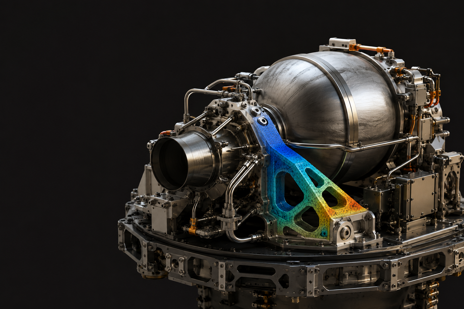
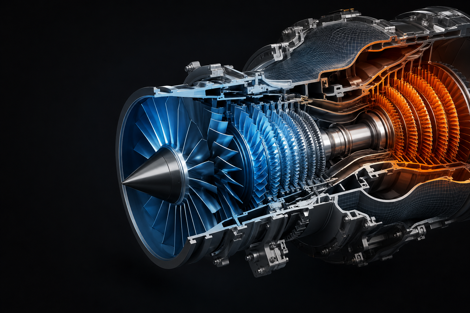
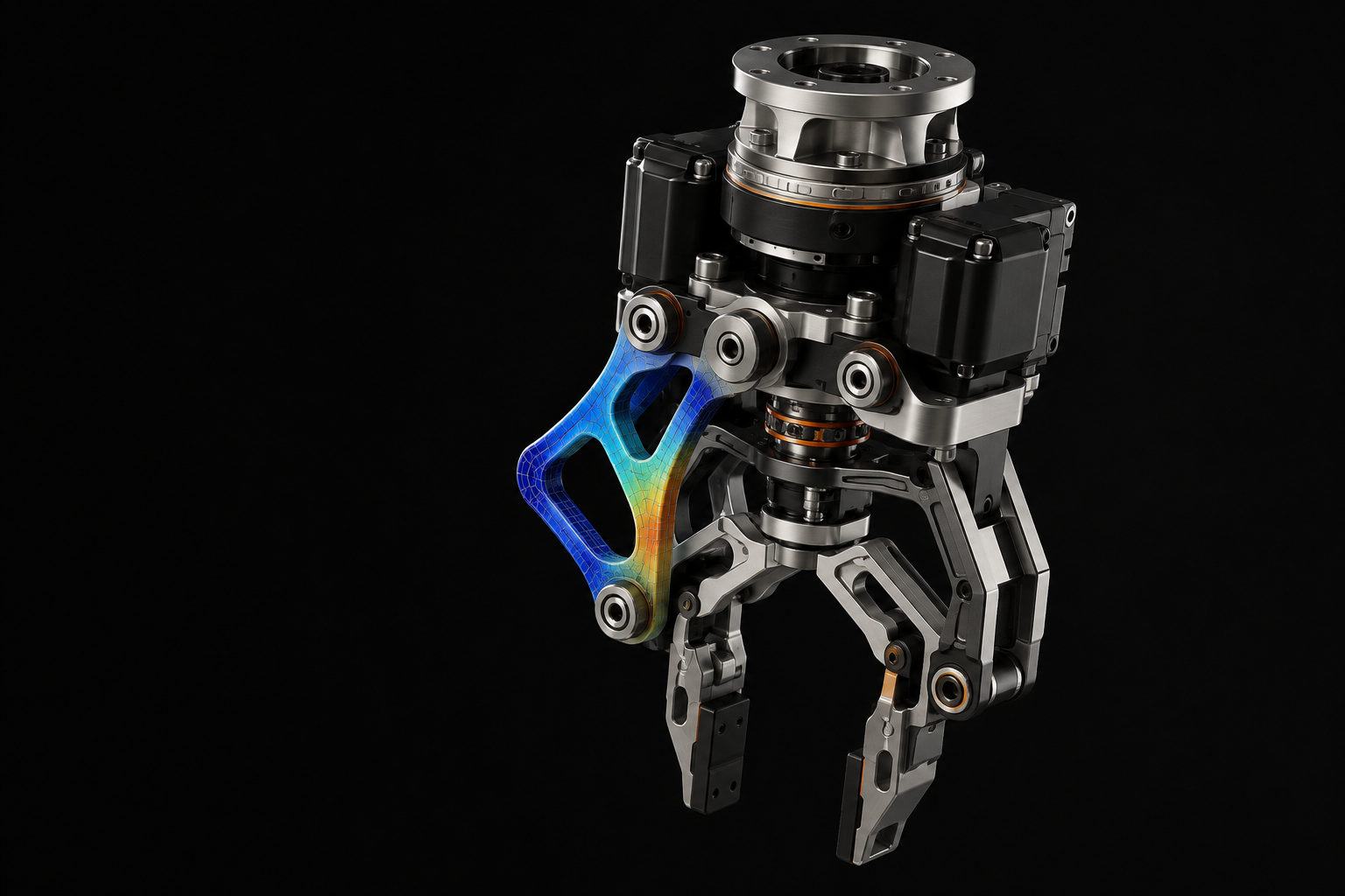
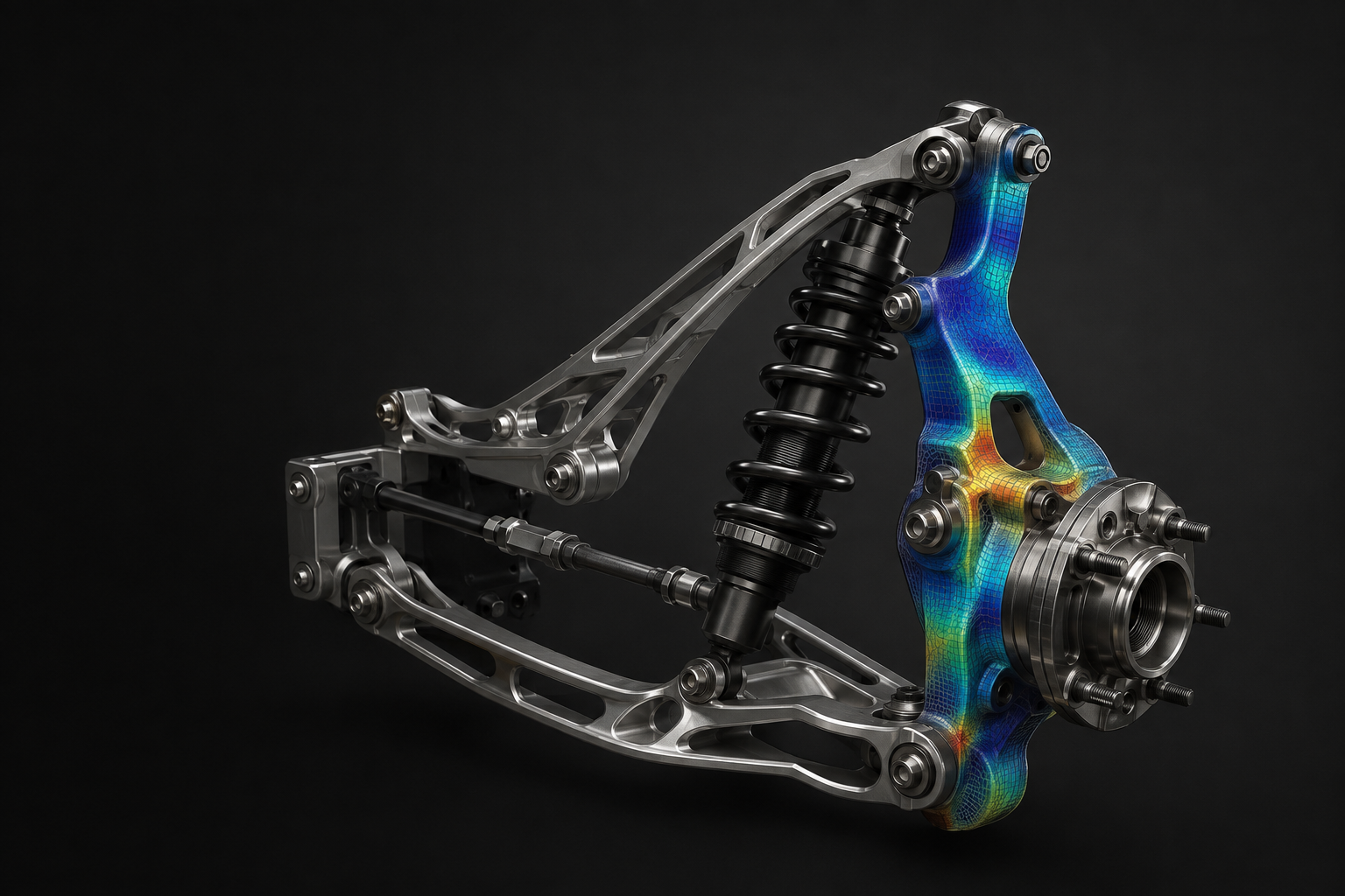
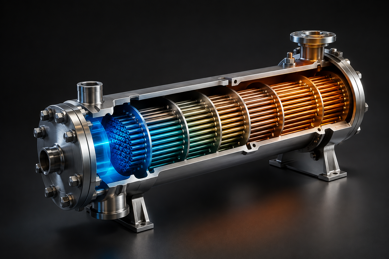
Wind, stress and heat stay attached to the model an agent can change and run again.
POST /v1/import

file       2020_corner_bracket.step
material   6061-T6 aluminium
load       100 N lateral
analysis   static

→ CAD imported
→ mesh             194 nodes · 501 tet4
→ peak stress       110 MPa
→ safety factor     2.18
→ equilibrium       balanced
→ mesh assessment   refinement advised
→ model bundle      ready
Simulation should be
seen as evidence.
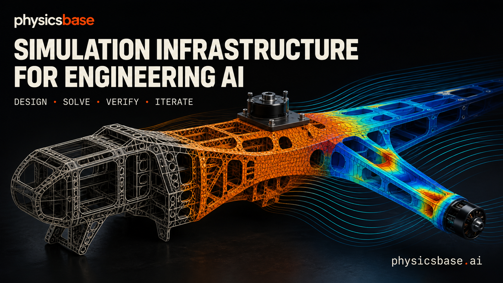
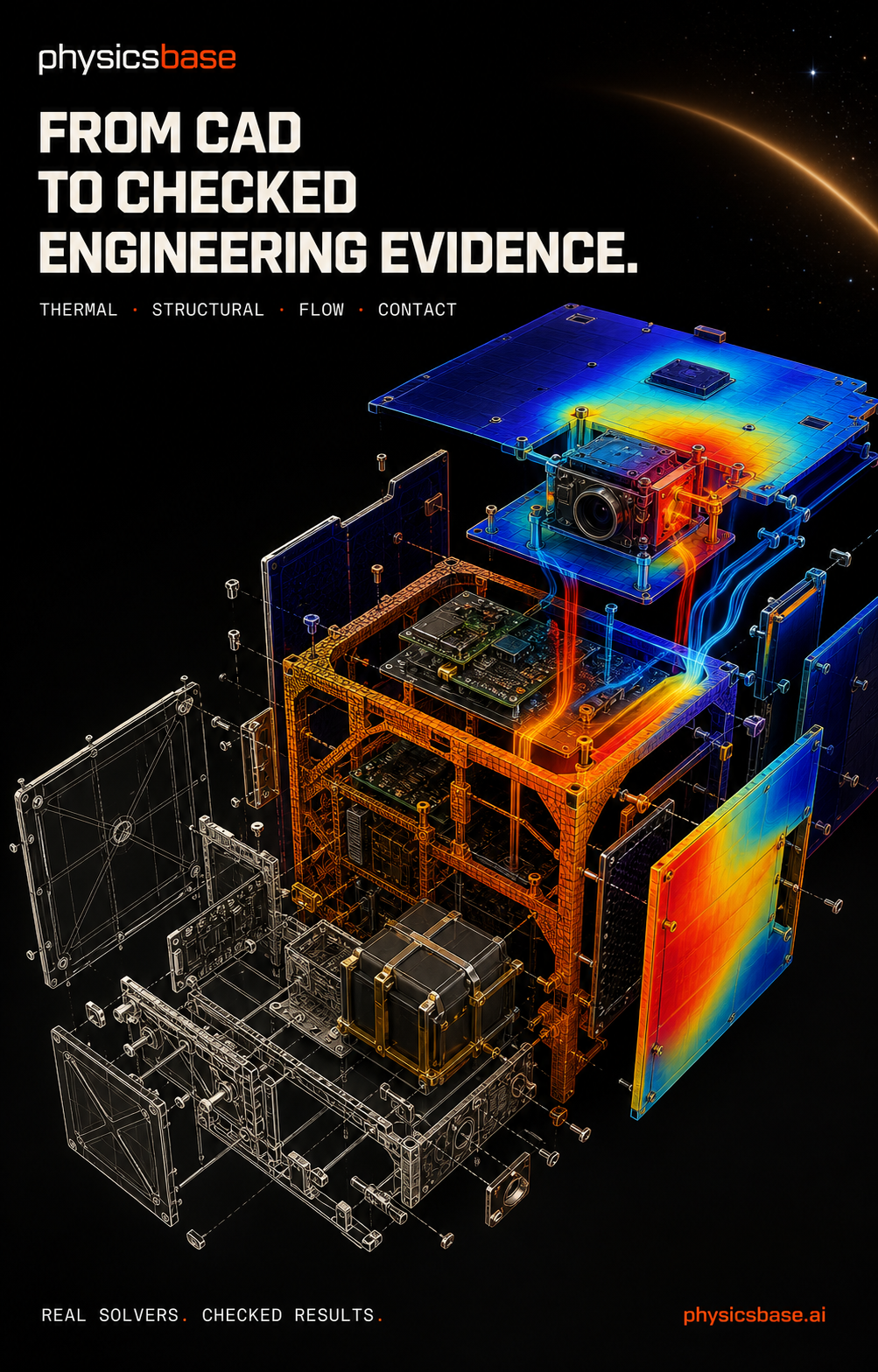
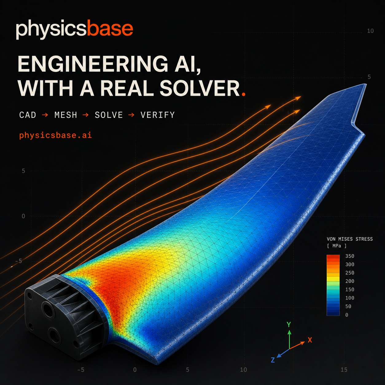
Real geometry, visible assumptions and fields you can inspect. Three views of the same idea: engineering AI needs more than an answer—it needs the solved model.
An expert FEA agent
that runs the solver.
Not a chatbot that guesses. Describe a structure and a question in plain language; Copilot plans the analysis, calls the real verified physicsbase solver, and answers in SI units — with the PASS/REVIEW verdict and the reference it was checked against. It returns the solved model itself: an interactive contour with the boundary conditions, loads and material properties drawn and labeled — switch result fields, toggle the mesh or deformed shape, hover the legend to isolate a stress band, and hover the model to read values at any node.
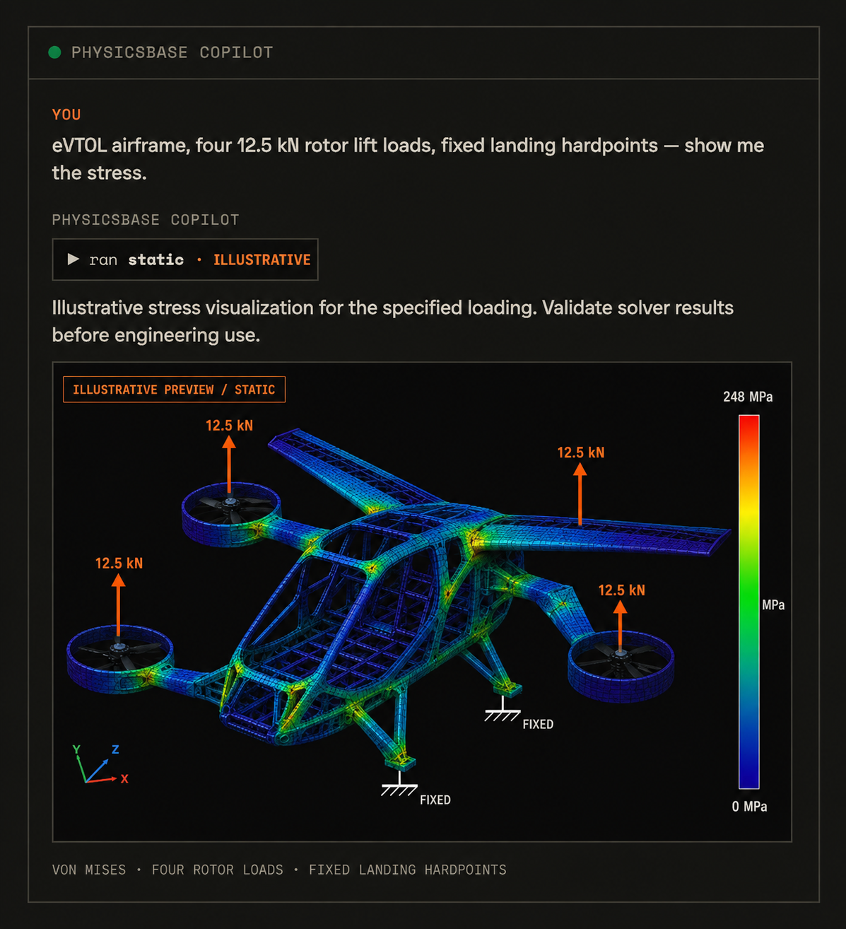
An agent can propose a design.
physicsbase lets it test one.
Create the model it actually needs.
Generate geometry or mesh connectivity, choose materials and sections, set supports, contacts and loads, then decide whether to stop, verify or iterate.
Get a computed model back—not a dead-end report.
Meshing, assembly, solution, result recovery and scoped checks return through one contract, together with a reusable model for the agent's next decision.
Run a real model
on the live server.
Solve a real model on the live server.
Pick a problem, adjust the input, then run the real server solve and inspect the returned model. No key is required.
Ready to run the complete server-side solve.
See the engine solve
the difficult cases.
ELEMENT VEHICLE MODEL
Automotive crash, with claim boundaries
Inspect the million-element Camry reference, the interrupted OpenRadioss impact trace, and exactly what is—and is not—solver output.
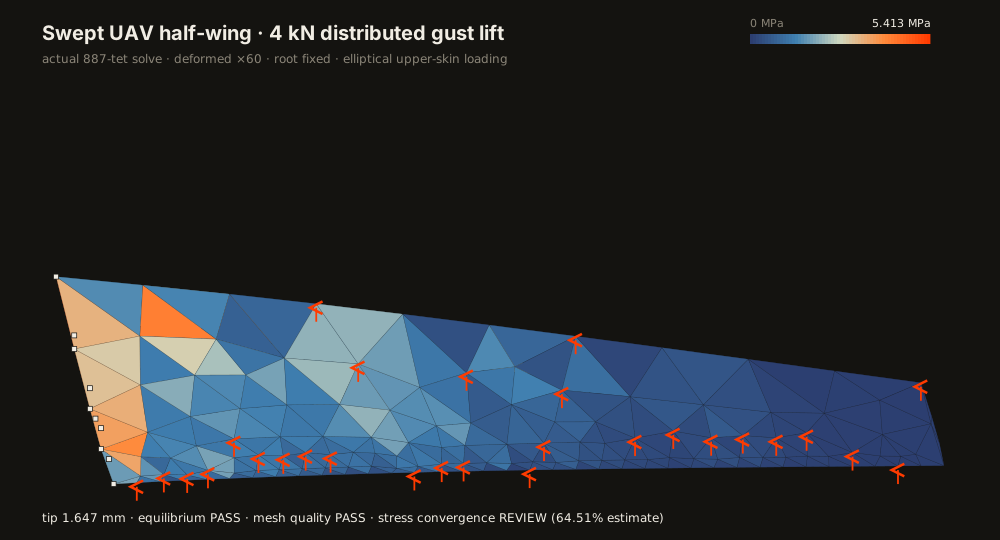
A gust load mapped onto real CAD
Mesh a swept UAV wing STEP and apply an elliptical lift law over its upper surface.
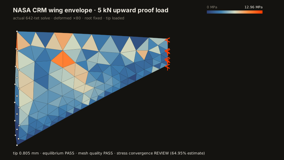
A real wing CAD, solved live
Trace an official NASA STEP through a bounded tetrahedral proof-load solve.
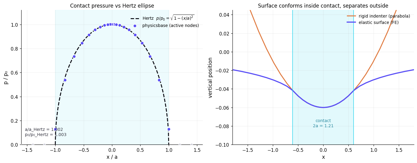
Contact without penalty tuning
Recover the Hertz pressure ellipse with an exact active-set solver.
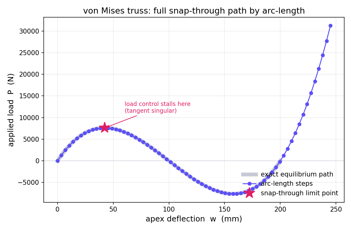
Past the limit point
Follow snap-through with Crisfield arc-length continuation.
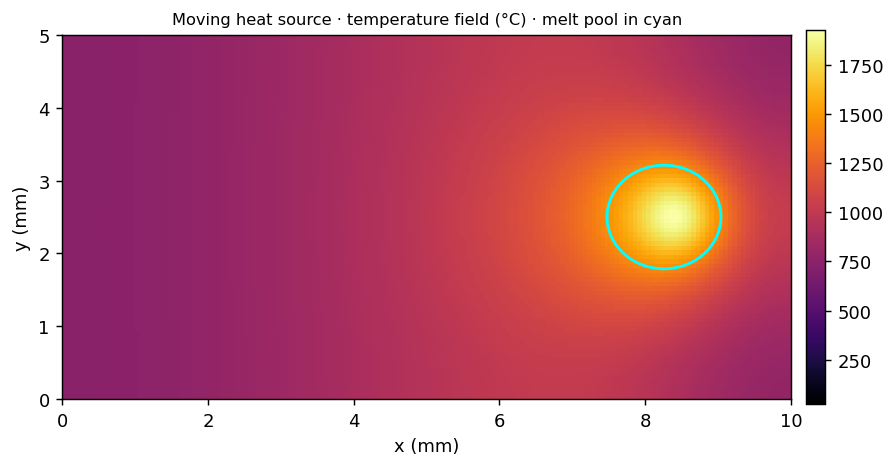
A moving heat-source field
Reproduce the melt-pool temperature field against the Rosenthal solution.
One contract for a single answer
or an entire design loop.
Loads, motion and stability.
Statics, modal, buckling, harmonic response, transient dynamics and prestressed modes.
When linear assumptions end.
Plasticity, contact, friction, hyperelasticity, large displacement and arc-length continuation.
Heat and transport.
Conduction, diffusion, moving heat sources, one- or two-way coupled thermo-mechanical response and acoustic cavity modes.
Predict, grow and optimize.
Damage, XFEM, phase-field fracture, progressive composite failure, stress-life fatigue and topology optimization.
From members to solids.
Bars, beams, frames, 2D and 3D solids, plates, shells and scalar-field elements.
Author it or bring it.
Submit agent-created nodes and elements directly, or import CAD, Abaqus, Nastran, Gmsh, VTK, STL and other engineering formats.
staticLinear statics — displacements, reactions, stressmodalNatural frequencies and mode shapesbucklingLinear buckling, critical loadsprestress_modalStress-stiffened modes — frequencies under preloadnewdamped_modalComplex modes · Rayleigh + physical non-proportional dashpotsnewrotordynamicsGyroscopic rotor modes · Campbell diagram · critical speedsnewharmonicSteady-state frequency responsenewtransientNewmark time integrationexplicit_dynamicsCentral difference · nonlinear/plastic trusses + 3D solids · rigid-wall impactnewnltransientNonlinear dynamics — snap-through, large rotationnewplasticityvon Mises / J2 with hardeningdamage_plasticityDuctile damage-plasticity (Lemaitre)newfinite_plasticityLarge-strain J2 — trusses + 3D solids, log strainnewviscoelastic / creepProny relaxation · Norton power-law creepnewviscoplasticPerzyna overstress · rate-dependent J2newstokesViscous incompressible Stokes flownewnavier_stokesSteady Navier-Stokes (Picard/Oseen)newunsteady_navier_stokesTransient Navier-Stokes — Taylor-Green vortexnewhyperelasticNeo-Hookean · Mooney-Rivlin · Ogden · fibre / GOH dispersionnewnlgeomLarge-displacement geometryarclengthSnap-through past limit pointscontactRigid-barrier, deformable pairs, node-to-surface (non-matching)newfrictionCoulomb stick / slipnewstepsMulti-step load history (load/unload)adaptiveMakes the mesh finer until convergednewdamageNonlinear continuum damagetopologySIMP topology optimizationnewxfemEdge-crack stress-intensity factornewphasefieldBrittle fracture, crack growthnewfatigueS-N life · Miner · rainflownewcrack_growthParis-law crack growth to failurenewstrain_lifeε-N low-cycle (Coffin-Manson)newfatigue_fePer-element life from the FE stress fieldnewmoving_heatMoving heat source / melt poolnewacoustic_modes / responseCavity/duct modes · driven HelmholtznewpiezoelectricCoupled electro-mechanical bar (converse/direct)newvibroacousticStructure↔fluid coupled modesnewmagnetostatics2D magnetic vector potential (B = curl A)newfield.*Heat, diffusion, potential flow, transportcoupledThermo-mechanical (one/two-way)truss2d/3dBars, pin-jointed structuresbeam2dEuler-Bernoulli frametimo2dTimoshenko shear-deformable beamframe3dSpace frame: axial+torsion+biaxialcst / quad4Plane stress / strain continuumtri6 / quad8Higher-order plane elementstet4 / hex8 / hex8i3D solids, linear (hex8i = incompatible modes)newtet10 / hex203D solids, higher-ordernewaxiquad4Axisymmetric solid (r–z)plate4 / mitc4Plate bending (SRI / MITC4)newshell4 / shell_mitc4Flat shell (membrane+bending) · composite layup sectionsnewspringGrounded / linking springfield_*Scalar-field line / tri / quad / tet / heximportSTEP / IGES / BREP · Abaqus .inp · Nastran · Gmsh · VTK · STLnewEvery result comes with
reasons to trust it.
Hertzian contact
Contact half-width and peak pressure against Hertz's analytical solution.
Scordelis-Lo roof
The standard shell benchmark matches the published reference displacement.
Snap-through path
Arc-length continuation follows the equilibrium path through the limit point.
Numerical Verification Guide
1314 executed comparisons, correctly identified as 368 case definitions.
Physical Validation Status
Zero qualifying experiments. See the evidence required before that claim can change.
Benchmark Guide
Inspect each published target, mesh history, fixed tolerance and convergence history.
From design intent
to the agent's next decision.
Create or import.
Generate geometry or finite elements directly, or start from STEP, IGES, BREP, Abaqus, Nastran, Gmsh, VTK or STL data.
Express the intent.
Set materials, sections, supports, contacts, loads, analysis settings, requirements and design variables.
Mesh, solve and check.
physicsbase builds the numerical model, runs the analysis and evaluates the checks supported for that analysis.
Use the model again.
Inspect fields, reactions, provenance and evidence; then change the returned bundle, compare it or re-submit it.
Use it once—or make it
the agent's design loop.
One-time simulation. Verification gate. Optimization engine.
Connect an engineering copilot, autonomous design workflow or simulation platform. The same editable model, computed fields and evidence travel through REST, MCP, OpenAPI and Python.
Open the integration guide →/llms.txtcompact discovery for language models/v1/capabilitiessupported analyses, elements and limits/openapi.jsontool schemas for agent frameworks/mcpnative tools for compatible agents/v1/importexisting CAD, mesh or solver data to simulation/v1/solveagent-authored model to checked, reusable resultBuilt to run big,
and to run for a long time.
Never assemble the stiffness.
The largest models are limited by the memory of the assembled global stiffness and the preconditioner built on top of it. The matrix free solver never forms that matrix. It applies the stiffness to a vector element by element, so working memory stays proportional to the number of unknowns rather than to the fill of a sparse factorization. It is verified to reproduce the assembled operator, its diagonal, and the direct solve to machine precision, in both the cached and the recompute modes.
Preconditioned conjugate gradients.
Above a size threshold the linear solve switches from a direct factorization to conjugate gradients with algebraic multigrid or incomplete LU preconditioning, and it falls back to a direct solve if the iteration stalls, so the caller always gets an answer. The matrix free path uses a Jacobi preconditioner assembled from the diagonal alone. Every result reports exactly which path ran under the same transparency rule as the physics self check.
Checkpoint, survive, resume.
A long solve writes its current iterate and its progress to disk while it runs. If the worker is killed or redeployed, the solve reloads its last checkpoint and warm starts the iteration instead of starting over. Because conjugate gradients converge monotonically, a resumed run reaches the same solution as an uninterrupted one, which is verified. Large problems can also be submitted as background jobs and polled, so no request blocks on a slow computation.
Exact model order reduction.
Guyan static condensation eliminates the interior unknowns of a model onto its boundary through the exact Schur complement, producing a superelement. Static condensation carries no approximation for linear statics, so the reduced solve reproduces the full solution to machine precision, with a symmetric and positive definite reduced stiffness and a matching strain energy.
Days and weeks of solves, with nac.
A single solve is one thing; a months long engineering program is another. physicsbase connects to nac, the open source agent harness from Arcee, over its public MCP endpoint. nac plans a campaign, decomposes it into threads that return structured episodes, and keeps every step aligned to the original intent while it fires many verified solves. It reads the verification verdict on each result and never advances the campaign on a failed check. physicsbase makes one solve scale and endure; nac makes a whole campaign of solves scale and endure.
The nonlinear path scales too.
The nonlinear and dynamic structural solvers now route their inner Newton tangent solves through the same iterative path as the linear static solve, so a large plasticity, large displacement, or nonlinear transient problem gets conjugate gradients above the size threshold, verified identical to a direct solve below it. The matrix free element loop can also split across a thread pool for on core parallelism, reproducing the serial result to rounding. Distributing the element loop across machines and GPUs is the next step, and its foundations, an assembly free operator and durable resumable jobs, are already in place.
What agents cannot ask
physicsbase to do yet.
General contact interfaces.
Self-contact; large-sliding surface-to-surface and mortar contact; frictional dynamic contact.
Broader nonlinear constitutive models.
Shipping: J2 plasticity (temperature-dependent yield), finite-strain J2, Perzyna viscoplasticity, Norton/J2 creep (truss, 2D plane stress/strain, 3D), Prony viscoelasticity, Ogden/Mooney-Rivlin/HGO/GOH hyperelasticity, Lemaitre damage-plasticity (trusses + continuum), combined isotropic+linear-kinematic (Prager) hardening, nonlinear (Armstrong-Frederick) kinematic hardening with a saturating back-stress and the Bauschinger effect, superposed multi-back-stress Chaboche hardening (bounded terms plus an unbounded linear ratcheting term), and Hill48 plane-stress anisotropic yield (calibrated from directional yields + Lankford R, verified to reduce to von Mises). Still open: full 3-D Hill with non-associative flow.
Advanced formulations.
Shipping: full unsymmetric laminate A/B/D coupling, top/bottom ply recovery with optional Hashin indices, ply-density consistent areal/rotary/coupled mass in both six-DOF shell formulations, axisymmetric rotating-disk/cylinder centrifugal stresses (solid and annular, plane stress or plane strain), Lame thick-walled pressure vessels (internal/external pressure), steady thermal-stress cylinders (logarithmic radial temperature gradient), axisymmetric Kirchhoff circular-plate bending (clamped or simply-supported, C¹ Hermite element), simply-supported rectangular-plate bending under the exact Navier sinusoidal load (locking-free MITC4), and Timoshenko shear-deformable beam deflection (bending + shear split, verified across slenderness ratios) — all verified against their exact closed forms. Still open: curved/degenerated and solid-shell elements; an analytic consistent tangent for continuum finite-strain plasticity.
Nonlinear crash and broader dynamic elements.
Shipping: truss/quad4 nonlinear implicit dynamics, complex modes with physical non-proportional dashpots, Euler-Bernoulli beam free-vibration frequencies (simply-supported, cantilever and clamped-clamped) and longitudinal rod natural frequencies (fixed-free, fixed-fixed and free-free), both verified against the exact closed form, linear frame-shaft gyroscopic rotordynamics with Campbell critical speeds, and native explicit central differences with spectral/CFL step enforcement, linear elastic waves, co-rotational elastoplastic trusses, total-Lagrangian elastoplastic first-order 3D solids and kinematic rigid-wall impact. Still open: beam/shell nonlinear explicit dynamics; rate effects, damage/failure, shell folding and deformable/self-contact in explicit crash; nonlinear rotor effects, centrifugal prestress, cross-coupled bearings and unbalance response.
Mixed-mode growth and life prediction.
Shipping: stress-life (Basquin S-N, Miner, Goodman/Soderberg/Gerber, rainflow), Paris-law crack growth, strain-life (Coffin-Manson-Morrow) fatigue, and cohesive-zone delamination (bilinear mode-I and mixed-mode I/II with the Benzeggagh-Kenane criterion, verified against the fracture energy Gc). Still open: mixed-mode KI/KII separation with crack-tip enrichment; crack-path tracking as a service; embedding cohesive elements between arbitrary faces in a full mesh.
Viscous CFD and FSI.
Shipping: viscous incompressible Stokes, full steady Navier-Stokes with convection, and transient (unsteady) Navier-Stokes (stabilized Q1-Q1), verified vs Poiseuille, Kovasznay and the Taylor-Green vortex; plus inviscid potential flow and scalar transport. Still open: turbulence models; free-surface flow; fluid-structure interaction.
Beyond CLT and staggered coupling.
Shipping: two-way thermo-mechanical coupling and field-coupled thermo-elasto-plasticity; piezoelectricity (1D bar plus 2D/3D coupled continua); acoustics (cavity/duct modes, driven + damped Helmholtz response) and vibro-acoustic structure↔fluid coupling; magnetostatics (linear + nonlinear saturable B–H); time-harmonic eddy currents; full-wave (scalar) time-harmonic electromagnetics with losses; Biot poroelastic consolidation (coupled displacement–pore-pressure column, verified against Terzaghi's exact consolidation series); and hygro-mechanical moisture swelling (Fickian uptake driving an isotropic swelling eigenstrain, verified against the restrained/free-bar closed forms). Still open: 3D woven RVEs, full WWFE envelopes, interlaminar/free-edge response, fully monolithic (single-Jacobian) coupling, the full vector (edge-element) Maxwell system and waveguide dispersion, 3D wetted-interface vibro-acoustic coupling, and transient/fully-coupled hygro-thermal response.
Production geometry automation.
Feature-aware sizing and quality controls for agent-authored geometry; full solver-deck assembly fidelity; p-refinement; contact-aware and boundary-layer meshes; remeshing surface-only 3D files.
Large nonlinear and distributed solves.
Shipping: a matrix-free element-by-element static solver that never assembles the global stiffness (O(n) memory, Jacobi-preconditioned CG, verified against the assembled operator and the direct solve to machine precision); durable checkpointed jobs that resume exactly after interruption for hours-long runs; and Guyan static condensation / superelements (exact Schur-complement reduction onto retained boundary DOFs). Still open: iterative routing beyond static analysis; parallel, distributed and GPU assembly/solve; general model-order reduction (POD/Craig-Bampton dynamic superelements) and multi-substructure assembly.
Decision-grade uncertainty and validation.
Nonlinear spatial and nonlinear-dynamic time error estimators; multi-level and 3D contact convergence beyond today's opt-in two-grid check; goal-oriented error; uncertainty quantification; stable targeted refinement; a qualified experimental campaign. Physical validation is not established today.
Give your engineering agent
a real simulation loop.
Start with one solve. Keep going through verification, comparison and optimization with the complete model returned after every run. The live example needs no key.