Chasing a melt pool.

A laser sweeping across metal leaves a tiny, blindingly hot pool that trails a comet of heat behind it. It's the physics at the heart of welding and 3D-printed metal — and it's a moving, transient heat-transfer problem. We solved it on physicsbase's field engine and checked it against the textbook.

Point a laser at a metal plate and drag it. Where the beam sits, the metal melts; a millimetre behind, it's already re-solidifying; a few millimetres away, it's barely warm. That travelling hot spot — the melt pool — governs everything about a weld or a 3D-printed part: its strength, its residual stress, whether it cracks. Predicting its temperature field is one of the workhorse problems of thermal engineering, and it's genuinely hard, because the heat source moves and nothing is ever in steady state in the lab frame. This is the moving-heat-source problem (Rosenthal 1946; and a staple of the additive-manufacturing FEM literature), and it maps cleanly onto physicsbase's transient field engine.

The problem

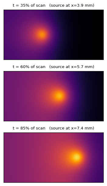
One equation governs it: \[ \rho c\,\frac{\partial T}{\partial t} \;=\; \nabla\!\cdot\!(k\,\nabla T) \;+\; Q(x, y, t) \] Heat capacity stores energy, conduction spreads it, and a source \(Q\) pumps it in — except here \(Q\) is a Gaussian blob that moves, its centre sliding across the plate at the scan speed. Everything interesting comes from the race between how fast the source moves and how fast heat can diffuse away from it. Move slowly and the field is nearly circular; move fast and it smears into the comet tail.

Using physicsbase: two operators and a time march

The finite-element ingredients are exactly two element matrices, and physicsbase hands back both from the same FieldQuad4 element that solves ordinary heat conduction. The conductivity operator is the spatial (diffusion) term; the capacitance operator is the transient (storage) term:

from femengine.field.elements import FieldQuad4

Ke = FieldQuad4.conductivity(cell, k,     {})   # (4,4)  ∫∇N·k∇N   — conduction
Ce = FieldQuad4.capacitance(cell, rho_c, {})   # (4,4)  ∫N·ρc·N    — heat storage
Fc = FieldQuad4.source(cell, 1.0,   {})   # (4,)   ∫N         — source template

Assemble those into global matrices K and C once, and the transient problem becomes a march in time. We use backward Euler, which is unconditionally stable — important, because the steep gradient at the source would make an explicit scheme explode. The clean part: the system matrix never changes, so we factorise it a single time and reuse the factorisation for all ~3000 steps.

# backward Euler:  (C/dt + K) T_new  =  (C/dt) T_old  +  F(t)
lu = splu((C/dt + K).tocsc())          # factorise ONCE — the matrix is constant

for step in range(nsteps):
    x_src = x0 + v*step*dt                # move the source this step
    Q_e   = Q0 * exp(-r2(x_src) / (2*r0**2))   # Gaussian at each element
    F     = assemble_source(Fc, Q_e)      # re-deposit the heat at its new spot
    T     = lu.solve(C/dt @ T + F)       # ← the only thing that changes each step

What came out

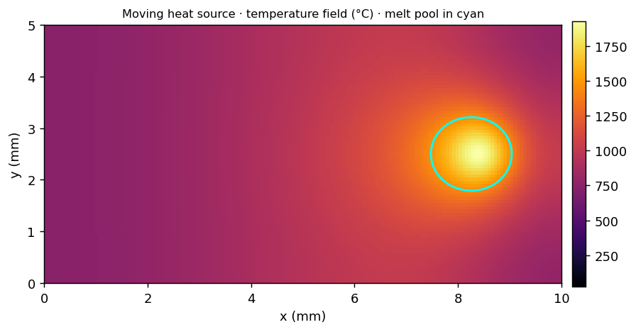
We swept a 180 kW/m line source across a 10 × 5 mm steel plate at 6 mm/s. The field is unmistakable: a searing peak of 1927 °C under the source, a compact melt pool (the region above steel's ~1450 °C melting point), and warmth trailing behind as the source pulls away.

Checking it against Rosenthal

In 1946 Rosenthal wrote down the exact temperature field for a moving point/line source in an infinite body — still the reference every moving-source code is measured against. Taking a slice along the scan line and plotting it in the source's moving frame, physicsbase reproduces Rosenthal's shape faithfully:

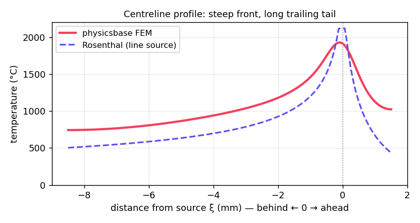
The two agree where it counts and differ exactly where they should. physicsbase is smoother right at the peak, because our source has a finite radius and the mesh a finite size, while Rosenthal's is a mathematical singularity. And our far tail runs a little warmer, because our plate is finite and insulated — it hangs onto heat that Rosenthal's infinite body carries away to infinity. Neither is a discrepancy; both are the physics of the boundary conditions.

Honest footnotes

This is the linear, single-phase version of the problem, which is enough to reproduce the melt-pool shape and validate against Rosenthal cleanly. It leaves out what the specialised additive-manufacturing codes add: the latent heat absorbed and released as metal melts and freezes, temperature-dependent conductivity and specific heat, convection in the liquid pool, and the third dimension. Those refinements move the numbers; they don't change the machine underneath — the same two FieldQuad4 operators, marched in time. That was the point: a general heat solver, pushed into a demanding moving-source regime, lands on the textbook answer.

References

1. D. Rosenthal, "The theory of moving sources of heat and its application to metal treatments," Transactions of the ASME 68 (1946), 849–866.
2. "Numerical simulation of transient heat conduction with a moving heat source using Physics-Informed Neural Networks" (2025). arXiv:2506.17726
3. "Modeling melt pool geometry in metal additive manufacturing" (2024). arXiv:2404.08834